Lemniskatische Konstante

Die lemniskatische Konstante ist eine 1798 von Carl Friedrich Gauß eingeführte mathematische Konstante. Sie ist definiert als der Wert des elliptischen Integrals

${\displaystyle \varpi =2\int _{0}^{1}{\frac {\mathrm {d} t}{\sqrt {1-t^{4}}}}}$ = 2,62205 75542 92119 81046 48395 89891 11941 36827 54951 43162 … (Folge A062539 in OEIS)

und tritt bei der Berechnung der Bogenlänge der gesamten Lemniskate von Bernoulli auf. Derzeit (Stand: 18. Juli 2022) sind 1.200.000.000.100 Nachkommastellen der lemniskatischen Konstante bekannt. Sie wurden von Seungmin Kim berechnet.

Bezeichnung

Gauß wählte für die lemniskatische Konstante bewusst die griechische Minuskel ${\displaystyle \varpi }$ (gesprochen: Skript-Pi oder Varpi), eine alternative Schreibweise von ${\displaystyle \pi }$, um an die Analogie zum Kreis mit seinem halben Umfang

${\displaystyle \pi =2\int _{0}^{1}{\frac {\mathrm {d} t}{\sqrt {1-t^{2}}}}}$

zu erinnern. Den Ursprung dieser Bezeichnung bei Gauß klärte vermutlich zuerst Ludwig Schlesinger auf: Zunächst verwendete Gauß zur Bezeichnung der lemniskatischen Periode das Zeichen ${\displaystyle \Pi }$, und ab Juli 1798 verwendete er für diese Größe konsequent ${\displaystyle {\tfrac {\varpi }{2}}}$.

Im Englischen findet sich für die Minuskel ${\displaystyle \varpi }$ auch die (irreführende) Bezeichnung pomega, ein Kofferwort aus den Buchstabennamen für π und ω.

Im englischen Sprachraum wird

${\displaystyle G=\varpi /\pi }$ = 0,83462 68416 74073 18628 14297 32799 04680 89939 93013 49034 … (Folge A014549 in OEIS)

als Gaußkonstante bezeichnet.

Herleitung der Integraldefinition

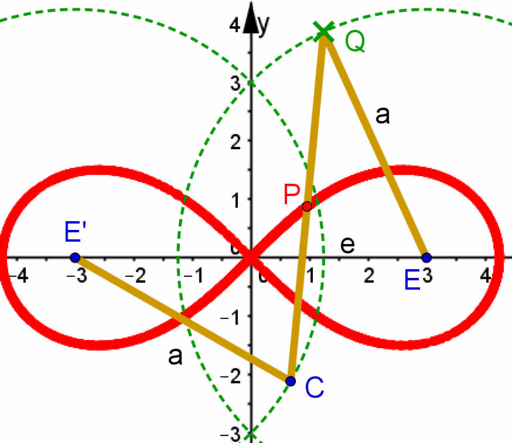
Folgende kartesische Koordinatengleichung ist für die Lemniskate von Bernoulli mit der Brennweite f gültig:

${\displaystyle (x^{2} y^{2})^{2}=2f^{2}(x^{2}-y^{2})}$

Daraus resultiert nachfolgende Parametergleichung für die Lemniskate mit dieser Brennweite:

${\displaystyle x(t)={\frac {{\sqrt {2}}f\sin(t)}{\cos(t)^{2} 1}}\quad \cap \quad y(t)={\frac {{\sqrt {2}}f\sin(t)\cos(t)}{\cos(t)^{2} 1}}\quad {\text{ mit }}\ 0\leq t<2\pi }$

Für das gegebene Intervall von t wird die gesamte Kurve der Lemniskate genau einmal parametrisiert. Der Umfang wird durch Integration von denselben Grenzen für t von der Pythagoräischen Summe der ersten Ableitungen bezüglich t berechnet:

${\displaystyle {\begin{aligned}U&=\int _{0}^{2\pi }{\sqrt {{\biggl (}{\frac {\mathrm {d} }{\mathrm {d} t}}x(t){\biggr )}^{2} {\biggl (}{\frac {\mathrm {d} }{\mathrm {d} t}}y(t){\biggr )}^{2}}}\ \mathrm {d} t\\&=\int _{0}^{2\pi }{\sqrt {{\biggl (}{\frac {\mathrm {d} }{\mathrm {d} t}}\cdot {\frac {{\sqrt {2}}f\sin(t)}{\cos(t)^{2} 1}}{\biggr )}^{2} {\biggl (}{\frac {\mathrm {d} }{\mathrm {d} t}}\cdot {\frac {{\sqrt {2}}f\sin(t)\cos(t)}{\cos(t)^{2} 1}}{\biggr )}^{2}}}\ \mathrm {d} t\\&=\int _{0}^{2\pi }{\sqrt {{\biggl (}{\frac {{\sqrt {2}}f\cos(t)[3-\cos(t)^{2}]}{[\cos(t)^{2} 1]^{2}}}{\biggr )}^{2} {\biggl (}{\frac {{\sqrt {2}}f[3\cos(t)^{2}-1]}{[\cos(t)^{2} 1]^{2}}}{\biggr )}^{2}}}\ \mathrm {d} t\\&=\int _{0}^{2\pi }{\frac {{\sqrt {2}}f}{\sqrt {\cos(t)^{2} 1}}}\ \mathrm {d} t=4\int _{0}^{\pi /2}{\frac {{\sqrt {2}}f}{\sqrt {\cos(t)^{2} 1}}}\ \mathrm {d} t=4\int _{0}^{\pi /2}{\frac {{\sqrt {2}}f}{\sqrt {\sin(t)^{2} 1}}}\ \mathrm {d} t\\&=4\int _{0}^{1}{\biggl [}{\frac {\mathrm {d} }{\mathrm {d} x}}\arcsin(x){\biggr ]}{\frac {{\sqrt {2}}f}{\sqrt {1 x^{2}}}}\ \mathrm {d} x=4\int _{0}^{1}{\frac {{\sqrt {2}}f}{\sqrt {1-x^{4}}}}\ \mathrm {d} x\end{aligned}}}$

Der maximale Durchmesser der Lemniskate von Bernoulli beträgt ${\displaystyle 2{\sqrt {2}}f}$ und die lemniskatische Konstante ist als Quotient des Vollumfangs dividiert durch den maximalen Durchmesser definiert:

${\displaystyle \varpi ={\frac {U}{2{\sqrt {2}}f}}=2\int _{0}^{1}{\frac {1}{\sqrt {1-x^{4}}}}\,\mathrm {d} x}$

Eigenschaften

Eulersche Betafunktion

Mit der Eulerschen Betafunktion ${\displaystyle \mathrm {B} }$ und der Gammafunktion ${\displaystyle \Gamma }$ gilt

${\displaystyle \varpi ={\tfrac {1}{4}}{\sqrt {2}}\,\mathrm {B} ({\tfrac {1}{4}},{\tfrac {1}{4}})={\tfrac {1}{2}}\,\mathrm {B} ({\tfrac {1}{4}},{\tfrac {1}{2}})=\Gamma ({\tfrac {1}{4}})^{2}/{\bigl (}2{\sqrt {2\pi }}{\bigr )}.}$

Deswegen gilt auch das Folgende:

${\displaystyle \int _{0}^{\infty }e^{-x^{4}}\mathrm {d} x={\frac {{\sqrt[{4}]{\pi }}\cdot {\sqrt {\varpi }}}{2\cdot {\sqrt[{4}]{2}}}}}$

Dirichletsche Betafunktion

Ebenso kann die lemniskatische Konstante mit der Ableitung der Dirichletschen Betafunktion auf folgende zwei Weisen dargestellt werden:

${\displaystyle \varpi =\pi ^{1/2}\exp {\bigl [}\beta '(0){\bigr ]}}$

${\displaystyle \varpi =2^{-1/2}\pi \exp \left[{\frac {1}{2}}\,\gamma -{\frac {2}{\pi }}\beta '(1)\right]}$

Das Kürzel ${\displaystyle \gamma }$ drückt hierbei die Euler-Mascheroni-Konstante aus.

Dabei gilt nach der Abel-Plana-Formeldefinition für die Dirichletsche Betafunktion:

${\displaystyle \beta (x)={\frac {1}{2}} \int _{0}^{\infty }{\frac {\sin[x\arctan(y)]}{2\,(y^{2} 1)^{x/2}}}\operatorname {csch} {\bigl (}{\frac {\pi }{2}}\,y{\bigr )}\,\mathrm {d} y}$

Und somit gilt für die Ableitung der Dirichletschen Betafunktion:

${\displaystyle \beta '(x)=\int _{0}^{\infty }{\frac {2\arctan(y)\cos[x\arctan(y)]-\ln(y^{2} 1)\sin[x\arctan(y)]}{4\,(y^{2} 1)^{x/2}}}\operatorname {csch} {\bigl (}{\frac {\pi }{2}}\,y{\bigr )}\,\mathrm {d} y}$

Unendliche Summen

Gauß fand die Beziehung

${\displaystyle \varpi =\pi /\operatorname {agm} (1;{\sqrt {2}})}$

mit dem arithmetisch-geometrischen Mittel agm und gab auch eine schnell konvergierende Reihe

${\displaystyle \varpi ={\frac {\pi }{\sqrt {2}}}\sum _{k=0}^{\infty }{\binom {2k}{k}}^{\!2}{\frac {1}{2^{5k}}}}$

mit Summanden der Größenordnung ${\displaystyle {\frac {1}{k2^{k}}}}$ an.

Außerdem erkannte Carl Friedrich Gauß folgenden Zusammenhang:

${\displaystyle \varpi =4\operatorname {arcsl} ({\tfrac {1}{2}}) 2\operatorname {arcsl} ({\tfrac {7}{23}})}$

${\displaystyle \varpi =\sum _{k=0}^{\infty }{\binom {2k}{k}}{\frac {1}{4^{k}(4k 1)}}{\biggl [}4\left({\frac {1}{2}}\right)^{4k 1} 2\left({\frac {7}{23}}\right)^{4k 1}{\biggr ]}}$

Dabei wird mit ${\displaystyle \operatorname {arcsl} }$ der Lemniskatische Arkussinus ausgedrückt.

Weitere Arcussinus-Lemniscatus-Summen von diesem Schema können so erzeugt werden:

${\displaystyle \varpi =4\operatorname {arcsl} (a) 2\operatorname {arcsl} \{\tan[{\tfrac {1}{4}}\pi -2\arctan(a^{2})]\}}$ mit ${\displaystyle 0\leq a\leq 1}$

Die Auswertung

${\displaystyle \varpi =2\sum _{k=0}^{\infty }{\binom {2k}{k}}{\frac {1}{(4k 1)2^{2k}}}}$

des elliptischen Integrals ergibt eine ähnliche Reihe, die jedoch sehr viel langsamer konvergiert, da die Glieder von der Größenordnung ${\displaystyle {\frac {1}{k^{3/2}}}}$ sind. Sehr schnell konvergiert die Reihe in

${\displaystyle \varpi =\pi {\biggl [}\sum _{k=-\infty }^{\infty }(-1)^{k}\,e^{-\pi k^{2}}{\biggr ]}^{2}={\frac {\pi }{\sqrt {2}}}{\biggl [}\sum _{k=-\infty }^{\infty }\,e^{-\pi k^{2}}{\biggr ]}^{2}}$

mit Summanden der Größenordnung ${\displaystyle e^{-\pi k^{2}}}$.

Auch sehr schnell konvergiert folgende Reihe:

${\displaystyle \varpi ={\frac {\pi }{\sqrt {2}}}\sum _{k=-\infty }^{\infty }\operatorname {sech} (\pi k)}$

Niels Nielsen stellte 1906 mit Hilfe der Kummerschen Reihe der Gammafunktion einen Zusammenhang mit der Eulerschen Konstante ${\displaystyle \gamma }$ her:

${\displaystyle \log \varpi ={\tfrac {1}{2}}\gamma -{\tfrac {1}{2}}\log 2 \log \pi {\frac {2}{\pi }}\sum _{k=1}^{\infty }(-1)^{k}{\frac {\log(2k 1)}{2k 1}}}$

Theodor Schneider bewies 1937 die Transzendenz von ${\displaystyle \varpi }$. Gregory Chudnovsky zeigte 1975, dass ${\displaystyle \Gamma (1/4)}$ und somit auch ${\displaystyle \varpi }$ algebraisch unabhängig von ${\displaystyle \pi }$ ist.

Unendliche Produkte

Analog zum Wallisschen Produkt lassen sich für die lemniskatische Konstante folgende Produktreihen entwickeln:

${\displaystyle \varpi =2\prod _{k=0}^{\infty }{\frac {(4k 3)(4k 4)}{(4k 2)(4k 5)}}={\sqrt {2}}\prod _{k=0}^{\infty }{\frac {(4k 2)(4k 4)}{(4k 1)(4k 5)}}}$

Folgende Produktreihen konvergieren sehr schnell:

${\displaystyle \varpi =\pi \prod _{k=1}^{\infty }\tanh(\pi k/2)^{2}={\frac {\pi }{\sqrt[{4}]{2}}}\prod _{k=1}^{\infty }\tanh(\pi k)^{2}}$

Elliptische Integrale

Vollständige elliptische Integrale K und E

Mit dem vollständigen elliptischen Integral erster Art lässt sich die lemniskatische Konstante auf verschiedene Weise darstellen:

${\displaystyle \varpi ={\sqrt {2}}K\left({\frac {1}{\sqrt {2}}}\right)=4({\sqrt {2}}-1)K[({\sqrt {2}}-1)^{2}]={\sqrt[{4}]{27}}({\sqrt {3}}-1)K\left[{\frac {1}{2}}({\sqrt {3}}-1)({\sqrt {2}}-{\sqrt[{4}]{3}})\right]=}$

${\displaystyle =8({\sqrt {2}} 1)^{2}({\sqrt[{4}]{2}}-1)^{2}K[({\sqrt {2}} 1)^{2}({\sqrt[{4}]{2}}-1)^{4}]=5{\sqrt {2}}({\sqrt {5}}-2)K\left[{\frac {1}{\sqrt {2}}}({\sqrt {5}}-2)(3-2{\sqrt[{4}]{5}})\right]}$

Die lemniskatische Konstante kann auch ausschließlich mit Ellipsenumfängen und somit mit elliptischen Integralen zweiter Art dargestellt werden:

${\displaystyle \varpi =(2 {\sqrt {2}})E[({\sqrt {2}}-1)^{2}]-2E\left({\frac {1}{\sqrt {2}}}\right)=}$

${\displaystyle ={\frac {3}{2}}(2{\sqrt {2}} {\sqrt {6}}-{\sqrt[{4}]{27}}-{\sqrt[{4}]{3}})E\left[{\frac {1}{2}}({\sqrt {3}}-1)({\sqrt {2}}-{\sqrt[{4}]{3}})\right]-{\frac {1}{2}}(3{\sqrt[{4}]{3}} {\sqrt[{4}]{27}}-3{\sqrt {2}})E\left({\frac {1}{\sqrt {2}}}\right)}$

Dabei ist E(k) das Verhältnis des Viertelumfangs zur längeren Halbachse bei derjenigen Ellipse, bei welcher die numerische Exzentrizität den Wert k annimmt.

Liste bestimmter elliptischer Integrale erster Art

Folgende weitere Integrale involvieren die lemniskatische Konstante:

${\displaystyle \int _{0}^{1}{\frac {1}{\sqrt {x^{4} 1}}}\,\mathrm {d} x={\frac {\varpi }{2{\sqrt {2}}}}}$

${\displaystyle \int _{0}^{1}{\frac {1}{(1-x^{4})^{3/4}}}\,\mathrm {d} x={\frac {\varpi }{\sqrt {2}}}}$

${\displaystyle \int _{0}^{1}{\frac {1}{(1-x^{2})^{3/4}}}\,\mathrm {d} x=\varpi }$

${\displaystyle \int _{0}^{\infty }{\sqrt {\operatorname {sech} (x)}}\,\mathrm {d} x=\varpi }$

${\displaystyle \int _{0}^{\pi /2}{\sqrt {\operatorname {sec} (x)}}\,\mathrm {d} x=\varpi }$

Herleitung der elliptischen Integrale zweiter Art

Nach der Kettenregel gelten folgende vier Ableitungen:

${\displaystyle {\frac {\mathrm {d} }{\mathrm {d} x}}{\biggl (}\int _{0}^{1}{\frac {x}{\sqrt {1-x^{4}y^{4}}}}\,\mathrm {d} y{\biggr )}={\frac {1}{\sqrt {1-x^{4}}}}}$

${\displaystyle {\frac {\mathrm {d} }{\mathrm {d} x}}{\biggl (}\int _{0}^{1}{\frac {x^{3}y^{2}}{\sqrt {1-x^{4}y^{4}}}}\mathrm {d} y{\biggr )}={\frac {x^{2}}{\sqrt {1-x^{4}}}}}$

${\displaystyle {\frac {\mathrm {d} }{\mathrm {d} x}}{\biggl \{}{\frac {y^{2} 1}{2y^{2}}}{\biggl [}{\text{artanh}}{\bigl (}y^{2}{\bigr )}-{\text{artanh}}{\biggl (}{\frac {{\sqrt {1-x^{4}}}\,y^{2}}{\sqrt {1-x^{4}y^{4}}}}{\biggr )}{\biggr ]}{\biggr \}}={\frac {x^{3}(y^{2} 1)}{\sqrt {(1-x^{4})(1-x^{4}y^{4})}}}}$

${\displaystyle {\frac {\mathrm {d} }{\mathrm {d} y}}{\biggl [}\arctan(y)-{\frac {1-y^{2}}{2y}}{\text{artanh}}(y^{2}){\biggr ]}={\frac {y^{2} 1}{2y^{2}}}\operatorname {artanh} (y^{2})}$

Im Folgenden werden zwei Gleichungsketten synthetisiert und danach gleichgesetzt:

Der Hauptsatz der Differential- und Integralrechnung wird auf folgende Weise angewendet:

${\displaystyle \int _{0}^{1}{\frac {\mathrm {d} }{\mathrm {d} x}}{\biggl (}\int _{0}^{1}{\frac {x}{\sqrt {1-x^{4}y^{4}}}}\mathrm {d} y\int _{0}^{1}{\frac {x^{3}y^{2}}{\sqrt {1-x^{4}y^{4}}}}\mathrm {d} y{\biggr )}\mathrm {d} x=}$

${\displaystyle ={\biggl [}\int _{0}^{1}{\frac {x}{\sqrt {1-x^{4}y^{4}}}}\mathrm {d} y\int _{0}^{1}{\frac {x^{3}y^{2}}{\sqrt {1-x^{4}y^{4}}}}\mathrm {d} y{\biggr ]}_{x=0}^{x=1}=}$

${\displaystyle =\int _{0}^{1}{\frac {1}{\sqrt {1-y^{4}}}}\mathrm {d} y\int _{0}^{1}{\frac {y^{2}}{\sqrt {1-y^{4}}}}\mathrm {d} y={\frac {\varpi }{2}}\int _{0}^{1}{\frac {x^{2}}{\sqrt {1-x^{4}}}}\mathrm {d} x}$

Das Produkt folgender zwei Integrale lässt sich dann mit der Produktregel und dem Satz von Fubini auf folgende Weise umformen:

${\displaystyle \int _{0}^{1}{\frac {\mathrm {d} }{\mathrm {d} x}}{\biggl (}\int _{0}^{1}{\frac {x}{\sqrt {1-x^{4}y^{4}}}}\mathrm {d} y\int _{0}^{1}{\frac {x^{3}y^{2}}{\sqrt {1-x^{4}y^{4}}}}\mathrm {d} y{\biggr )}\mathrm {d} x=}$

${\displaystyle =\int _{0}^{1}{\biggl (}{\frac {1}{\sqrt {1-x^{4}}}}\int _{0}^{1}{\frac {x^{3}y^{2}}{\sqrt {1-x^{4}y^{4}}}}\mathrm {d} y {\frac {x^{2}}{\sqrt {1-x^{4}}}}\int _{0}^{1}{\frac {x}{\sqrt {1-x^{4}y^{4}}}}\mathrm {d} y{\biggr )}\mathrm {d} x=}$

${\displaystyle =\int _{0}^{1}\int _{0}^{1}{\frac {x^{3}(y^{2} 1)}{\sqrt {(1-x^{4})(1-x^{4}y^{4})}}}\,\mathrm {d} y\,\mathrm {d} x=\int _{0}^{1}\int _{0}^{1}{\frac {x^{3}(y^{2} 1)}{\sqrt {(1-x^{4})(1-x^{4}y^{4})}}}\,\mathrm {d} x\,\mathrm {d} y=}$

${\displaystyle =\int _{0}^{1}\int _{0}^{1}{\frac {\mathrm {d} }{\mathrm {d} x}}{\biggl \{}{\frac {y^{2} 1}{2y^{2}}}{\biggl [}{\text{artanh}}{\bigl (}y^{2}{\bigr )}-{\text{artanh}}{\biggl (}{\frac {{\sqrt {1-x^{4}}}\,y^{2}}{\sqrt {1-x^{4}y^{4}}}}{\biggr )}{\biggr ]}{\biggr \}}\,\mathrm {d} x\,\mathrm {d} y=}$

${\displaystyle =\int _{0}^{1}{\frac {y^{2} 1}{2y^{2}}}\operatorname {artanh} (y^{2})\,\mathrm {d} y=\int _{0}^{1}{\frac {\mathrm {d} }{\mathrm {d} y}}{\biggl [}\arctan(y)-{\frac {1-y^{2}}{2y}}{\text{artanh}}(y^{2}){\biggr ]}\mathrm {d} y=}$

${\displaystyle ={\biggl [}\arctan(y)-{\frac {1-y^{2}}{2y}}{\text{artanh}}(y^{2}){\biggr ]}_{y=0}^{y=1}=\arctan(1)={\frac {\pi }{4}}}$

Denn nach der Regel von de L’Hospital gilt:

${\displaystyle \lim _{y\rightarrow 0}{\frac {1-y^{2}}{2y}}{\text{artanh}}(y^{2})=0}$

${\displaystyle \lim _{y\rightarrow 1}{\frac {1-y^{2}}{2y}}{\text{artanh}}(y^{2})=0}$

Durch Gleichsetzung der beiden aufgestellten Gleichungsketten folgt:

${\displaystyle {\frac {\varpi }{2}}\int _{0}^{1}{\frac {x^{2}}{\sqrt {1-x^{4}}}}\mathrm {d} x={\frac {\pi }{4}}}$

${\displaystyle \int _{0}^{1}{\frac {x^{2}}{\sqrt {1-x^{4}}}}\mathrm {d} x={\frac {\pi }{2\varpi }}}$

Liste bestimmter elliptischer Integrale zweiter Art

Aus dem soeben gezeigten Endresultat lassen sich folgende Integrale herleiten:

${\displaystyle \int _{0}^{1}{\frac {\sqrt {x^{4} 1}}{(x^{2} 1)^{2}}}\,\mathrm {d} x={\frac {1}{4{\sqrt {2}}}}\left(\varpi {\frac {\pi }{\varpi }}\right)}$

${\displaystyle \int _{0}^{1}{\frac {x^{2}}{(x^{4} 1)^{3/2}}}\,\mathrm {d} x={\frac {\pi }{4{\sqrt {2}}\,\varpi }}}$

${\displaystyle \int _{0}^{1}{\frac {1}{(1-x^{2})^{1/4}}}\,\mathrm {d} x={\frac {\pi }{\varpi }}}$

${\displaystyle \int _{0}^{\infty }{\sqrt {\operatorname {sech} (x)^{3}}}\,\mathrm {d} x={\frac {\pi }{\varpi }}}$

Weitere bestimmte elliptische Integrale

Diese beiden elliptischen Integrale dritter Art sind zueinander identisch:

${\displaystyle \int _{0}^{\infty }{\frac {x^{2}}{(x^{2} 1){\sqrt {x^{4} 1}}}}\,\mathrm {d} x=\int _{0}^{\infty }{\frac {1}{(x^{2} 1){\sqrt {x^{4} 1}}}}\,\mathrm {d} x}$

In der Stammfunktion von der ersten Funktion bewirkt die Substitution von x durch die Kehrwertfunktion 1/x und die anschließende Negativsetzung die Bildung der Stammfunktion von der zweiten Funktion. Außerdem gilt folgende Aufsummierung:

${\displaystyle \int _{0}^{\infty }{\frac {x^{2}}{(x^{2} 1){\sqrt {x^{4} 1}}}}\,\mathrm {d} x \int _{0}^{\infty }{\frac {1}{(x^{2} 1){\sqrt {x^{4} 1}}}}\,\mathrm {d} x=\int _{0}^{\infty }{\frac {1}{\sqrt {x^{4} 1}}}\,\mathrm {d} x={\frac {\varpi }{\sqrt {2}}}}$

Daraus folgt:

${\displaystyle \int _{0}^{\infty }{\frac {x^{2}}{(x^{2} 1){\sqrt {x^{4} 1}}}}\,\mathrm {d} x={\frac {\varpi }{2{\sqrt {2}}}}}$

${\displaystyle \int _{0}^{\infty }{\frac {1}{(x^{2} 1){\sqrt {x^{4} 1}}}}\,\mathrm {d} x={\frac {\varpi }{2{\sqrt {2}}}}}$

Wie bereits oben erwähnt ist diese Integralformel gültig:

${\displaystyle \Gamma ({\frac {5}{4}})=\int _{0}^{\infty }\exp(-x^{4})\,\mathrm {d} x=2^{-5/4}\pi ^{1/4}\varpi ^{1/2}}$

Basierend auf dem Eulerschen Ergänzungssatz über die Gammafunktion hat folgendes Integralprodukt den nachfolgenden Wert:

${\displaystyle {\biggl [}\int _{0}^{\infty }\exp(-x^{4})\,\mathrm {d} x{\biggr ]}{\biggl [}\int _{0}^{\infty }x^{2}\exp(-x^{4})\,\mathrm {d} x{\biggr ]}={\frac {\pi }{8{\sqrt {2}}}}}$

Im Zusammenhang mit der Gammafunktion gilt somit jenes Integral:

${\displaystyle {\frac {1}{4}}\Gamma ({\frac {3}{4}})=\int _{0}^{\infty }x^{2}\exp(-x^{4})\,\mathrm {d} x=2^{-9/4}\pi ^{3/4}\varpi ^{-1/2}}$

Ellipsenumfang

Bei einer Ellipse, in welcher sich die größere Halbachse zur kleineren Halbachse in der Quadratwurzel aus Zwei verhält, nimmt das Verhältnis des Ellipsenumfangs zur kleineren Halbachse den Wert 2ϖ 2π/ϖ an. Diese Tatsache wird im nun Folgenden bewiesen:

${\displaystyle U/b=4{\sqrt {2}}E{\bigl (}{\frac {1}{\sqrt {2}}}{\bigr )}=4\int _{0}^{1}{\sqrt {{\bigl (}{\frac {\mathrm {d} }{\mathrm {d} x}}{\sqrt {2-2x^{2}}}{\bigr )}^{2} 1}}\,\mathrm {d} x=4\int _{0}^{1}{\sqrt {{\frac {2x^{2}}{1-x^{2}}} 1}}\,\mathrm {d} x=4\int _{0}^{1}{\frac {1 x^{2}}{\sqrt {1-x^{4}}}}\mathrm {d} x=}$

${\displaystyle =4\int _{0}^{1}{\frac {1}{\sqrt {1-x^{4}}}}\mathrm {d} x 4\int _{0}^{1}{\frac {x^{2}}{\sqrt {1-x^{4}}}}\mathrm {d} x=2\varpi {\frac {2\pi }{\varpi }}}$

Somit gilt für diese Ellipse:

${\displaystyle U=({\sqrt {2}}\varpi {\sqrt {2}}\pi \varpi ^{-1})a=(2\varpi 2\pi \varpi ^{-1})b}$

In dieser Tabelle werden mehrere Ellipsen mit ihren Umfangsverhältnissen aufgelistet:

Siehe auch

• Lemniskatischer Sinus
• Lemniskatischer Arkussinus
• Hyperbolisch lemniskatischer Sinus

Literatur

• Theodor Schneider: Einführung in die transzendenten Zahlen. Springer-Verlag, Berlin 1957, S. 64.
• Carl Ludwig Siegel: Transzendente Zahlen. Bibliographisches Institut, Mannheim 1967, S. 81–84.
• John Todd: The Lemniscate Constants. Institute of Technology, Kalifornien 1975
• A. I. Markuschewitsch: Analytic Functions. Kapitel 2 in: A. N. Kolmogorov, A. P. Juschkewitsch (Hrsg.): Mathematics of the 19th Century. Geometry, analytic function theory. Birkhäuser, Basel 1996, ISBN 3-7643-5048-2, S. 133–136.
• Jörg Arndt, Christoph Haenel: π. Algorithmen, Computer, Arithmetik. 2. Auflage, Springer, 2000, S. 94–96 (hier ist die griechische Minuskel ϖ typographisch korrekt wiedergegeben)
• Steven R. Finch: Gauss’ Lemniscate constant, Kapitel 6.1 in Mathematical constants, Cambridge University Press, Cambridge 2003, ISBN 0-521-81805-2, S. 420–423 (englisch)
• Hans Wußing, Olaf Neumann: Mathematisches Tagebuch 1796–1814 von Carl Friedrich Gauß. Mit einer historischen Einführung von Kurt-R. Biermann. Ins Deutsche übertragen von Elisabeth Schuhmann. Durchgesehen und mit Anmerkungen versehen von Hans Wußing und Olaf Neumann. 5. Auflage, 2005, Eintrag [91a].

Weblinks

• Eric W. Weisstein: Lemniscate Constant. In: MathWorld (englisch).
• Eric W. Weisstein: Gauss's Constant. In: MathWorld (englisch).
• Folge A062540 in OEIS (Kettenbruchentwicklung von ϖ)
• Folge A053002 in OEIS (Kettenbruchentwicklung von ϖ/π)

Einzelnachweise